8 Building-scale vs district-scale
In this chapter, we compare the results of an optimisation at the building-scale and at the district-scale. As a reminder, optimisation at building scale uses the decentralized method and optimisation at district scale uses the decomposed method. For the optimisation, we have chosen to focus solely on TOTEX minimisation because we have adopted an economic perspective of the individual, who is seen as a rational actor aiming to minimise his costs. The comparison of both approaches is done on the KPIs (key performance indicators) and on the installed capacity. There are six different KPIs:
- The self-sufficiency (SS) corresponds to the share of electricity demand, which can be covered by onsite generated electricity.
- The self-consumption (SC) corresponds to the share of the onsite generated electricity, which is consumed by the decentralized energy system itself.
- The photovoltaic curtailment (PVC) factor corresponds to the share of the total amount of PV energy that is curtailed from the PV generation.
- The grid usage (GU) describes the interaction with the grid with respect to the maximum uncontrollable load of the building. The uncontrollable load is excluding the demand for heating. Therefore, this indicator evaluates the impact of a system design on the grid. This indicator can be seen from two points of view: the supply (GUs) and the demand (GUd).
- The grid usage supply (GUs) represent the amount of power imported through the transformer divided by the maximal domestic electricity power used by the district.
- The grid usage demand (GUd) represent the amount of power exported through the transformer divided by the maximal domestic electricity power used by the district.
- The photovoltaic penetration (PVP) measures how much of the total electricity demand of the building and the units could be covered by generated electricity from photovoltaic panels.
- The levelized cost of electricity (LCoE) is the true cost of onsite consumed electricity. It respects also the investment in the energy system infrastructure. The used version (LCoE1) is balancing the cost of the electricity generated onsite.
In theory, the district approach, using the principle of pooling of energy balance by allowing exchanges between buildings, should be more efficient than the approach of optimising each building individually. Consequently, we except to see an improvement when adopting the district approach. Optimising the three districts produces unexpected results. Indeed, there is almost no variation in the KPIs and in installed capacity between both optimisation scales.
The comparison of TOTEX and GWP plots reveals minimal discrepancies in both CAPEX and OPEX, indicating that the results of the optimisation is the same for both cases. Furthermore, this analysis suggests that the installed capacity remains unchanged. Both Tables 8.1 and 8.2 confirm the visual result. There is no difference either in the KPIs or in the installed capacity. This analysis is done using the example of the Jonction district. The plots for the other two districts can be found in the appendix. The results are the same, i.e. the difference between the two types of optimisation is negligible.
Figure 8.1: TOTEX comparison between building and district scale of Jonction district
Figure 8.2: GWP comparison between building and district scale of Jonction district
| Scale | SC | SS | PVC | GUs | GUd | PVP | LCoE1 |
|---|---|---|---|---|---|---|---|
| Building | 0.436 | 0.428 | 0 | 2.06 | 4.41 | 0.982 | -0.108 |
| District | 0.437 | 0.429 | 0 | 2.06 | 4.42 | 0.981 | -0.108 |
| Scale | PV | Electrical Heater SH | Heat pump Air | Heat pump Geothermal | Water Tank SH | Electrical Heater DHW | Water Tank DHW |
|---|---|---|---|---|---|---|---|
| Building | 5798.55 | 590.87 | 0 | 1200.36 | 113.55 | 98.57 | 50.88 |
| District | 5792.75 | 590.88 | 0 | 1200.35 | 113.55 | 98.57 | 50.83 |
This lack of difference is a surprising result that can be explained by the current electricity retail and feed-in tariffs, as shown in Figure 8.3. This graph shows that with current tariffs, the best option is to install solar panels, regardless of the scale chosen for optimisation. Consequently, we can not see the attractiveness of pooling production and consumption on a TOTEX optimisation in a fully electric system. Moreover, considering the highly competitive feed-in price, the necessity for storage diminishes significantly when no other constraints except TOTEX minimisation is taken into account. This situation explains the lack of difference between the optimisations.
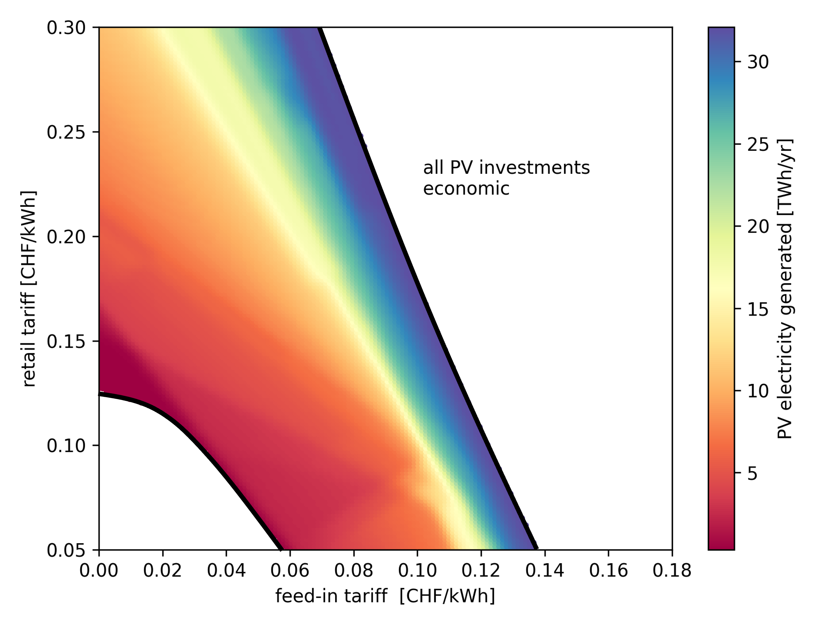
Figure 8.3: Rainbow plot of the PV installation regarding the feed-in and the retail tarif
In the following analyses, we focus on the district scale optimisation to demonstrate the advantages of energy communities.