6 Integration of stochasticity

In this chapter, we provide a comprehensive overview of the model, before presenting more specific considerations of the parameters employed.

6.1 Model

6.1.1 Explanation of SIA profiles

Currently, the model uses the SIA2024 standards to extract typical profiles for the electricity and hot water end use demand of a household. Moreover, the heat gains are calculated by adding the heat gains of the inhabitants and the electricity consumption. The plot below shows three daily SIA profiles and the calculated heat gains profiles.

Figure 6.1: Bar plot of the SIA profiles

6.1.2 Explanation of the modelisation of the stochasticity

To generate the end use demand of a district, REHO uses the SIA profiles and other information such as area, year of construction or class of each building. The SIA profiles imposes the distribution and the characteristics of each building impact this distribution. When working on a district, this way of generating the energy leads to a situation in which the consumption peaks are reached at the same time.

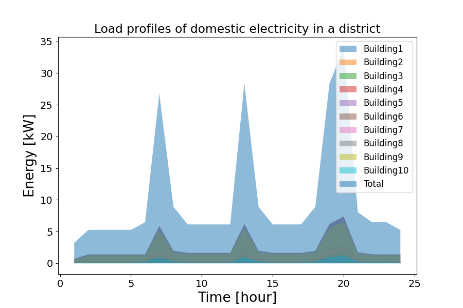
Figure 6.2: Electrical consumption of 10 buildings without stochasticity

Synchronisation of peaks is shown in Figure 6.2 for the electricity end use demand. We observe that the peaks are distributed as in Figure 6.1. Using this optimisation, we observe flatted part and peaks at specific time, which is not really closed to the reality. Due to the non-typical nature of individual behavior, making accurate predictions of the consumption can be challenging. Therefore, in order to make REHO more realistic, a stochastic effect has been incorporated into the SIA profiles.

To add stochasticity, two different operations are applied to the standard profiles. There is a random effect that allows for a variation in amplitude and a random effect that allows for a variation in time. Each building has his own stochastic effect.

Firstly, the amplitude variation is modelled by multiplying the typical profile by an amplitude factor. This factor need to be around the value of 1 and it is generated with a Gaussian distribution. This way of modeling allows to incorporate uncertainty and variability in the amount of electricity consumption. The amplitude factor can be an amplification or a reduction due to the symmetric bell-shaped curve of the Gaussian distribution. The standard deviation of the distribution determines the variability of the factor. The equation corresponding to the amplitude variation is:

\[\begin{equation} \text{Final}_{t} = a \cdot \text{Original}_{t} \end{equation}\] With \(|a|\) being the amplitude factor

Secondly, the time shift of the SIA profiles introduce a random shift, also called a lag to the original time series, effectively moving each data point forward or backward in time. This allows to apply a different random temporal displacements for each building of the district. The shift factor is also generated with a Gaussian distribution for the same reason than the amplitude variation. For this shift factor, the mean of the Gaussian distribution will be 0 and the standard deviation will determine the variability of the shift factor. This factor value can be positive or negative. A positive shift factor value indicate a forward shift and a negative factor indicate a backward shift.

\[\begin{equation} \text{Final}_{t} = \text{Original}_{t}* (1-|SF|)+\text{Original}_{t\pm1}*|SF| \end{equation}\] With \(|SF|\) being the shift-factor

In Figure 6.3, the same district as in 6.2 is optimised with this stochastic effect that implies a time shift for each building of the district. We observe that the peaks are more smooth than before and that the phasis between these peaks are less flat. The total load is spread over a time interval. This situation corresponds more to the reality as not all individuals are using electricity at the same time.

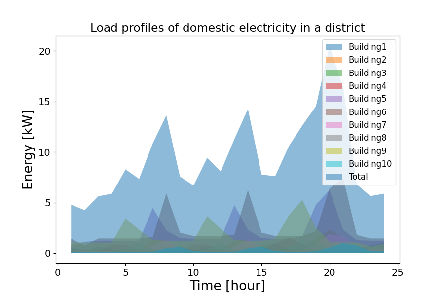
Figure 6.3: Electrical consumption of 10 buildings with stochasticity

The differences between both situations is clearly noticeable on Figure 6.4. We clearly see the impact of the stochastic effect on the curve. The noticeable observation lies in the distinct disparity between the peaks. In the absence of the stochasticity effect, the intensity of the peaks is 30 kW. However, when the stochasticity effect is introduced, this peak level is no longer sustained. As a consequence of incorporating stochasticity, the phases between peaks become more variable, resulting in a less flat phases. Consequently, the variation between the lowest consumption points and the peak moments becomes less pronounced when stochasticity is considered. In comparing the total load, we observe that the intensity of the peaks is 30% less important than before.

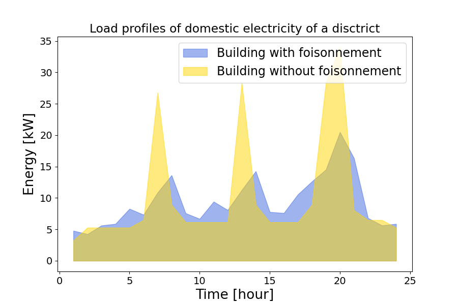
Figure 6.4: Comparison a load profiles of domestic electricity of a district with and without stochasticity in the standard profiles

6.2 Parameters

The Gaussian distribution is a symmetric distribution characterized by two parameters, the mean and the standard deviation. The concept of standard deviation with respect to the mean is a measure of the dispersion or variability of the data points around the mean. It represents the average amount by which individual data points deviate from the mean. In other words, it provides information about how much the data points are likely to deviate from the mean value. It quantifies the spread of the data and influences the shape of the distribution. The larger the standard deviation, the more dispersed the data is, so the further away from the mean. On the contrary, a small standard deviation implies that the data are close to the mean.

The empirical rule, also known as the three-sigma rule, is a guideline that describes the approximate proportions of data within certain ranges of standard deviations from the mean. Approximately 68% of the data falls within one standard deviation of the mean, 95% falls within two standard deviations, and about 99.7% falls within three standard deviations.

The standard deviation is an important parameter because it reflects the variability in the behaviour of the data considered. Indeed, assuming that the behaviour of individuals in buildings is homogeneous, it is necessary to set a small standard deviation. On the contrary, if heterogeneity is the hypothesis, the standard deviation will be greater.

In this study, we make the assumption that both the amplitude factor and the time shift factor follow Gaussian distributions. For the amplitude factor, the aim is to apply a multiplication factor to the consumption intensity. This distribution is centered around \(1\), ensuring that the average behavior is not affected by this factor. We fix the standard deviation at \(0.1\), as we assume a low variability in the consumption intensity. Regarding the time shift factor, we assume a standard normal distribution, meaning that the mean is \(0\) and the standard deviation is \(1\). The purpose of centering the distribution around \(0\) is to model all hours with the same Gaussian. By setting the standard deviation to \(1\), we ensure that there are approximately \(68\%\) values between \(-1\) and \(1\). The underlying assumption behind this choice is that the behaviors are relatively heterogeneous.