5 Energy community modeling

In order to estimate what would be the impact of creating a CEL for the different stakeholders of a neighborhood, a modeling of a CEL is realized in order to estimate the energetic fluxes between each participant to the CEL. In this present work, it has been decided, by SIG and IPESE, that the model would represent the eco-neighborhood of Les Vergers. This choice was mainly made because Les Vergers is a GIREC neighborhood and the eco-neighborhood of Les Vergers is a subset of this neighborhood for which synthetic load curve can be easily estimated.

Once the energetic fluxes between participants are known, financial fluxes between each stakeholders can be associated through pricing for different scenarii, and determine business models for the CEL.

5.1 Context : eco-neigborhood Les Vergers

The eco-neighborhood of Les Vergers is composed of 34 buildings which are mostly residential buildings : 30 out of 34 have SIA380/1 (société Suisse des Ingénieurs et des Architectes, meaning in english Swiss society of Engineers and Architects) class I (collective housing), 3 have class IV (schools) and one has class XI (sport infrastructure). The annual heating demand is about 7403 MWh, the annual cooling demand 29 MWh (note that only schools have a cooling demand), the annual Domestic Hot Water (DWH) demand is 1799 MWh and the annual electrical demand 4161 MWh.

The entire of the thermal needs of the 34 buildings are covered by a centralized 5 MWth heat pump (HP). Electrical needs come from the grid or PV panels installed on top of each building. There is no centralized nor personal battery nor geothermal source of energy. 3 of the buildings operates in simple RCP : the electricity locally produced by their PV panels can be self-consumed at the level of the building. For the other buildings, the locally produced electricity from PV panels is only used for common facilities (common lighting, elevator, etc.) such as the self-sufficiency rate of these buildings is between 3 and 4%.

5.2 Model

The model has been realized on REHO (Renewable energy hub optimizer), a decision support tool for energy system design, and using the QBuildings database. Both tools have been developed at IPESE.

In order to model the centralized heat pump that powers the eco-neighborhood, an AMPL model has been created to model properly the energetic exchanges inside the neighborhood.

Finally parameters of REHO have been adjusted in order to represent as much as possible the real energy system of the neighborhood.

5.2.1 REHO & QBuildings

The purpose of REHO is to optimize energy systems at building-scale or neighborhood-scale, considering simultaneously the optimal design as well as optimal scheduling of capacities. It allows to investigate the deployment of energy harvesting and energy storage capacities to ensure the energy balance of a specified territory, through multi-objective optimization and KPIs parametric studies.

It exploits the benefits of two programming languages: AMPL and Python.

• The core optimization model is written in AMPL: objectives, constraints, modeling equations (energy balance, mass balance, heating cascade etc.).
• All the input and output data is passed to the model through a Python wrapper. This data management structure is used for initialization of the optimization model, execution, and results retrieval

QBuildings is a Geographic Information System (GIS) database for the characterization of the territory from an energy point of view (end-use demand, building stock, endogenous resources). This database is built by gathering different public databases and combining them with SIA norms (SIA 2024 and SIA380/1).

5.2.1.1 Weather Data

REHO uses clustered weather data (irradiance and external temperature) to reduce the computational complexity of optimization. Instead of using the weather data of the 365 days a the year, it uses only weather data of 10 typical days for a year : each of the 365 is assigned to a typical day so that a synthetic time-series can be reproduced for the whole year for irradiance and the external temperature.

Together with these 10 days, 2 extremes periods, both of 1h, are extracted form the clustering algorithm. These 2 periods are used only for sizing of the energy conversion units to be installed for a building or a neighborhood : the units need to satisfy the demand for these extreme periods even though these periods are not used for the construction of the synthetic weather data time-series of one year.

Finally, only 242 (10*24 + 2) data points are used instead of 8760.

5.2.2 District heat pump

In REHO, energy harvesting technologies can be installed to equip a single building or a neighborhood. If a technology needs to be fed with a resource, it is model in REHO with an object called layer, with a type, for the type of resource the technology needs, and a time series with the amount of this resource the technology needs in order to meet its demand across time. Similarly, this technology feeds, as output, another layer that eventually represents the needs of a building.

The district heat pump is modeled in a way that it powers multiple heating network that are each connected to a building. In this model the heat pump is powered by the electricity layer and, in turn, powers a heat layer which feeds the unit demand of every heating network of each building. A model for heating district network existed already, therefore only a model for the district heat pump was to be developed.

5.2.3 Parameters

5.2.3.1 Global parameters

REHO has a plenty of parameters that can be adapted to fit more precisely a situation or to run an optimization with different objectives and constraints. In this present case, it is worth to note few important points that were determinant for choosing the right value for some parameters.

First the optimization has been run in order to optimize the entire neighborhood simultaneously. Therefore the parameter centralized was set to True. The Dantzig-Wolfe decomposition implemented in REHO for reducing the computational complexity was not needed here. Indeed, since the district heat pump fulfills the thermal need of the whole neighborhood, the complexity of the problem is reduced significantly and a centralized optimization can be run in an acceptable amount of time.

Second, the objective function has been set to the operational expenditure (OPEX) of the energy system of the neighborhood. The total expenditure (TOTEX), the sum of the operational and capital expenditure (CAPEX) was first chosen. However, the choice of energy harvesting technologies had been restricted in order to force REHO to install PV panels, the district heat pump and DHNs for each buildings. The sizing of the district heat pump was also restricted in order to have a heat pump of at least 3MWth. Thus, and given the used unit prices (the prices given by IPESE), optimizing the TOTEX or the OPEX doesn’t make a difference on the presence of these units in the energy system of the neighborhood. Since the district heat pump meets the thermal needs of the whole neighborhood, the optimization can only decide to install other units that provides electricity to the neighborhood, thus private batteries or a district battery. However, these units have a high CAPEX and are often not selected to be part of the energy system when optimizing the TOTEX. In order to analyses the leverage of a district battery in the neighborhood, it was then decided to optimized the OPEX rather than the TOTEX.

Third stochasticity was implemented in order to represent the stochastical behavior of the demand of the 34 building of the neighborhood. Stochasticity is implemented in REHO with the use of a normal distribution with 0-mean which represent the time shift of the energy demand or heating gain due to an occupancy profile of the building. Hence the standard deviation of the normal distribution has also to be set. Figure 5.1 shows the daily profile of one building of the neighborhood and 5.2 shows the the daily profile of the electrical demand of every buildings inside the neighborhood, with and without stochasticity implemented.

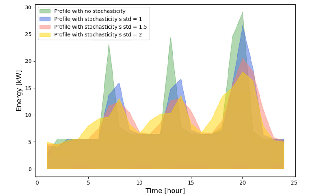
Figure 5.1: Daily electrical profile of one building of the neighborhood.

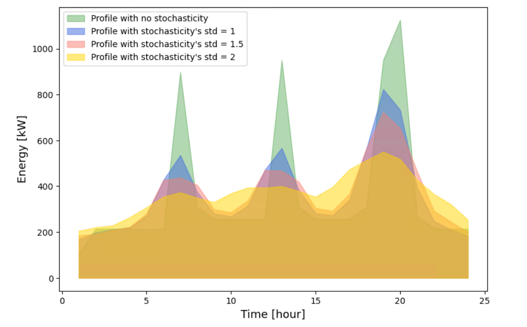
Figure 5.2: Daily electrical profile of the entire neighborhood

It has been decided that the profile that best represented the profile of the neighborhood was the one when the standard deviation of the normal distribution was set to 1.5h. This means that in a window of 1.5 standard deviations around a point t of the load curve, thus 1h and 30minutes hours before and after t, 68% of the buildings present this point in their new load curve.

5.2.3.2 Technical parameters

Every model of each energy harvesting technology present parameters that can also be changed.

In this present case, the COP of the district heat pump has been set to 3.69, the average annual COP of the HP according the Geneva’s university who has conducted a feedback analysis (Schneider, Brischoux, and Hollmuller, n.d.) on the energy system of Les Vergers. Moreover, surface capacity of the PV panels has been set to 0.162 \(kW/m^2\), the reference surface used in the feedback analysis.

5.3 Pricing

Once the data relative to energetic flows are extracted from the REHO model, and processed, the financial analysis is undertaken. The first step is to establish prices for each energetic flows. Since in the neighborhood the whole thermal demand has been electrified thanks to the district heat pump, the focus has been put on electrical pricing.

This section present the tariffs of the electrical demand that have been used for the financial model of the CEL of Les Vergers. The tariffs for electricity coming from the grid in Geneva, set by SIG whose activities include running the local DSO of Geneva and being a energy supplier, are presented but also the tariffs that could be established in a simple RCP (with no microgrid) and within a CEL.

5.3.1 SIG tariff

SIG runs the sole DSO of Geneva but plays also a role of energy supplier. Because of unbundling policies, these two activities are separated. SIG offers different tariffs for its customers and remunerate PV panels owners by buying their electricity production.

5.3.1.1 Electricity tariffs

Subscription depends on the amount of energy a customer annually consumes and on the annual maximal power it requires. In this study, three tariffs have been investigate : the simple low voltage tariff (BT simple), the professional low voltage tariff (proBT), and the professional medium voltage tariff (MT5). These tariff are presented in Appendix 11.

Professional tariffs are offered once the annual energy consumption reaches the threshold of 30’000 kWh. These tariffs present both a energy component and a power component, whereas the BT simple tariff only charges the energy component of the demand. Moreover, both of them are indexed on hours which are split between peak hours (PH) and off-peak hours (OPH) and depend as well on the season. There are therefore 4 prices for each tariff : PH in summer, OPH in summer, PH in winter and OPH in winter (Note that winter is considered to last from the 1st of october to the 31st of March, and summer from the 1st of April to the 30th of September). The billing is done on a monthly basis and is computed as followed :

(energy consumption during PH) * (energy price during PH) + (energy consumption during OPH) * (energy price during OPH) + (maximal annual power) * (power price)

For both of these tariffs, two optimal pricings are proposed, A or B, based on the annual power usage duration (DUP annuelle in french for Durée d’Utilisation de la Puissance annuelle) expressed in hours. This value is computed as followed : annual energy consumption/annual maximal power required. For these two tariffs, the optimal price is selected as followed :

• For the tariff proBT : if the DUP is above 3000h the optimal price selected is the B price which charges more the power component of the demand but less the energy component.
• For the tariff MT5 : if the DUP is above 3600h, similarly the optimal price selected is the B price which charges more the power component of the demand but less the energy component.

All these tariffs include federal and communal taxes as well as distribution charges. The DSO of SIG is rewarded with the distribution charges which include charges on the energy demand (per kWh) and charges on power demand (per kW). On the other hand, the energy supplier is rewarded with charges on the energy demand. The structure of the tariffs is the following :

• Energy supplier’s price of electricity (per kWh)
• Energy component of the distribution charges (per kWh)
• Power component of the distribution charges (per kW) - for professional tariffs only
• federal and communal taxes on the energy demand (per kWh)
• Communal taxes on the power demand (per kW) - for professional tariffs only

These 3 tariffs were used as a parameter of the REHO model : one optimization was made per tariff. However, as the price of the energy component of electricity is a scalar parameter in REHO (1-dimensional) and since both professional tariffs (proBT and MT) vary between PH and OPH, a mean price for these tariffs were used. The mean price was computed with a weighted mean of the price of energy over the 8760 hours of the year. The weights used were the amount of electricity need by the entire neighborhood for each hour of the year. The two mean prices \(p_{energy}\) for the energy component of electricity were thus the followings :

• \(p_{energy}^{proBT} = 0.179\) \(CHF/kWh\)
• \(p_{energy}^{MT} = 0.1603\) \(CHF/kWh\)

Note that only the energy component of the price of electricity varies between PH and OPH. The power component is constant across the year and is modelized in REHO by a monthy grid connection cost.

5.3.1.2 Remuneration policies

It is mandatory for SIG due to the Federal act on energy (Swiss Federal Assembly 2016), to buy electricity from PV production in its service area. The energy supplier of SIG offers therefore remuneration tariff for PV panels owner that injected electricity on its network. This tariff is composed only with a energy component but the DSO of SIG pays also a remuneration if the injection is done on the LV network

5.3.2 RCP tariff

The pricing terms may vary from one RCP to another based on their specificities, supply contracts, energy sources utilized, and other local factors. However prices schemes are established by following some directives, especially by taking into account the following components :

• Generation costs: The costs associated with electricity generation, including investment, operation, and maintenance of the assets.
• Grid usage and charges: The fees for using the grid infrastructure are factored into the pricing.
• Administrative and service fees: Depending on the RCP structure and contractual arrangements, administrative fees and service charges may be incorporated into the electricity prices.
• Local regulations and taxes: Any local regulations, policies, or taxes specific to the region .

One important directive is that the PV panels owner cannot charges the clients above a certain threshold which is equal to the mean between the price the client would pay its electricity if outside the RCP and the internal cost of PV panels. The internal cost of PV panels represent the annualized capital expenditure, operation and maintenance fees, the distribution and the billing fees. An illustration of this directive is presented in figure 5.3 where the PV panels internal cost is 16 cts/kWh and the electricity price outside the RCP 20 cts/kWh. Here the PV panels owner charges the client with the maximum amount it can.

Figure 5.3: Example of teh developpement of the PV-generated electricity sells price within a RCP (source : (OFEN, Asloc, APF, AES 2021))

In this study, the PV panels internal price has been set to 14 cts/kWh for establishing the baseline scenario. And it has been assume that the client would pay the BT simple tariff for electricity if outside any grouping (RCP or CEL). This choice of 14cts/kWh was based on the costs calculated internally by GIS for various installations and on examples found in the literature (OFEN, Asloc, APF, AES 2021).

5.3.3 CEL tariff

As CEL are not yet legally allowed in Switzerland, new tariffs need to be invented. Here for this study, PV-generated electricity tariff inside the CEL has been set to the RCP tariff with an additional charges due to the usage of the DSO distribution network. This distribution charge is set to a certain percentage of the distribution charge of the BT simple tariff. For the baseline scenario, this percentage is set to 50%. The same distribution charge is added to the electricity sales price of the battery owner (see section 5.4.2.2)

5.4 Financial analysis

The financial analysis is the computation of a balancing sheets for each stakeholders involved in the energy system of the neighborhood for different scenarii.

5.4.1 Scenarii

9 scenarii were investigated : 9 because 3 grouping categories are investigated (No grouping, RCP simple, and CEL) with the 3 tariffs (BT simple, proBT and MT5).

• The scenario No grouping is a scenario were there is no structure for common self-consumption : there is no auto-consumption at any level. This scenario is a simplification of the actual organization at les Vergers : since there is only 3 simple RCP in the neighborhood and that other buildings have a self-sufficiency around 3%, simplifications have been made and the self-sufficiency of the whole neighborhood is considered negligible. Hence it is assumed that every single household is an end-user and covers all its needs by importing electricity from the grid. Note that consumption are nonetheless aggregated at the building level. This skews the results on the annual maximum power of each end-users and on revenues relative to power charge since aggregating takes advantages of the stochasticity of the demand inside a same building. This is not intentional but REHO gives no results at a smaller scale than the building scale.

• The scenario RCP simple is a grouping category where self-consumption is allowed only at the building level : in this configuration no exchange between buildings or toward the heat pump are allowed but the DSO sees each buildings as end-users and households benefits from stochasticity at the building level.

• The scenario CEL is the scenario where every kind of exchange are allowed using the network of the DSO, however, the DSO sees the whole neighborhood as a single end-user. The billing for each building and the heat pump is made internally. This allows to take advantage of the stochasticity of the demand of the 34 buildings and the heat pump : the sum of the annual maximum power on each buildings plus de heat pump is not equal to the annual maximum power of the CEL. Power charge needs afterward to be split between the buildings and the heat pump. This is done by weighing power charges of the CEL by the percentage of contribution to the maximum power.

Additionally to these 9 scenarii, other scenarii where district units are installed, such as monodirectional Electrical Vehicles (EV) chargers and district battery, were also considered. EV were added because in the coming years, mobility is about the become more and more electrified (OCEV 2017). It was then considered interesting to simulate what would be the energy needs of the neighborhood if all the vehicles inside of it were to be EV and what would be the benefit of having a CEL in this case. The district battery was added because it represents a mean of providing flexibility to the neighborhood : it allows to reduce the maximal power needed for the neighborhood by acting like a energy buffer provider. As such it reduces the power stress on the network.

EV were added to every scenarii previously introduced, augmenting the number of scenarii by 9. Regarding the battery, as the centralized battery usage make sens only if it can directly exchange energy with other entities inside the neighborhood, this technology was added only in scenarii with CEL grouping category. Thus 6 scenarii were added, and the total number of scenarii raised to 24. In scenarii with CEL grouping category, the billing associated with power charges for these two centralized technologies was done the same way it was done for buildings and the heat pump, by splitting the charges for the annual maximum power of the CEL between each contributor.

It is now important to note that some scenarii don’t represent a scenario that is possible in real life. For instance scenarii No grouping with tariff proBT or MT5 would never appear in real life since in a scenario No grouping every end-user are households (plus the heat pump) that would never benefit from proBT nor MT5 tariff. Similarly for the scenarii RCP with tariff BT simple or MT5 and the scenario CEL with tariff BT simple. However, it is though that it is still interesting to keep them in order to assess more easily the outcomes of being under one grouping category or tariff. Indeed it is therefore possible to assess the changes in grouping category separately from the change in tariff.

5.4.2 Stakeholders

In the present case of Les Vergers, 7 stakeholders have been identified :

• The renters
• the heat pump owner
• the PV panels owner
• the DSO
• the energy provider
• the EV chargers owner
• the centralized battery owner

5.4.2.1 EV chargers owner

As previously mentioned, in this study EVs are charged inside the neighborhood by monodirectional chargers without any smart charging. The daily charging profile of one EV of the neighborhood, given in figure 5.4 was imposed in REHO. This profile comes from SIG internal calculation of the daily demand of EVs in Geneva.

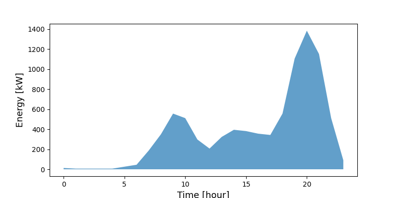
Figure 5.4: Charging profile of the electric vehicles

5.4.2.2 Battery owner

The district battery was added in some scenarii in order to have a mean to provide flexibility to the neighborhood. However, it is important to note that it is a technology that is very expensive in terms of investment. Based on SIG work, the price of a battery is given by : \(402\cdot x + 43507\) CHF where \(x\) is the capacity of the battery in kWh. Thus a battery of 1MWh for instance, would cost around 450kCHF.

Besides, the flexibility potential of the neighborhood offered by the battery, could in practice by offered by other cheaper means such as smart charging for the EV, leverage the thermal inertia of the buildings for thermal needs and the use of Energy Management Systems (EMS). EMS allow the renters of the neighborhood to manage their energy use. It helps identify opportunities to adopt and improve energy-saving strategies.

This is why it was decided to ignore the capital expenditure of the battery in the development of the energy sales price of the battery owner. Indeed, reporting the capital expenditure on this price would not make it attractive at all for consumers compared to the SIG price of electricity. This reflects the fact that a battery is usually not worth it when optimizing the TOTEX.

Equation (5.1) gives the energy sales prices \(p_{battery}\) [\(CHF/kWh\)] of the battery owner for which the economical viability of this stakeholder is ensured. Since in this present study, the second element of the right hand side of the equation is ignored, this stakeholder is therefore operating at a loss. Yet, this is not considered as an issue since the sole interest of the battery here is to provide flexibility which could be provided by other cheaper means, as already mentioned.

\[\begin{equation} p_{battery} = \frac{\text{OPEX}_{battery}}{E_{battery,y}} + \frac{\text{CAPEX}_{battery}/\tau}{E_{battery,y}} \tag{5.1} \end{equation}\]

Where :

• \(\text{OPEX}_{battery}\) [\(CHF/year\)] is the OPEX of the battery given by the cost of electricity the battery needs during an entire year. For professional tariffs, the mean price of the energy component of electricity, defined in section 5.3.1.1 was used and it was assumed that the battery owner would pay the monthly grid connection for every months of the year even if the battery doesn’t import electricity from the grid during certain months.

• \(\text{CAPEX}_{battery}\) [\(CHF\)] is the CAPEX of the battery;

• \(E_{battery,y}\) [\(kWh\)] is the annual amount of energy provided by the battery;

• \(1/\tau\) [\(year^{-1}\)] is the annualization factor given by : \(\frac{i\cdot(1+i)^n}{((1+i)^n -1)}\) with \(n\) [year], the lifetime of the battery and \(i\) [%] the interest rate. In this study \(n=10\) years and \(i=4\)%.

Since the size of the district battery can vary from one scenario to an other, the battery annual electricity needs would also vary from one scenario to an other and the energy sales price of the battery owner as well. For sake of simplicity, it has been decided to fix one common price for every scenarii. This common price \(p_{battery}^*\) is the mean price on the \(N_{battery}\) scenarii which include a battery. It is given by equation (5.2):

\[\begin{equation} p_{battey}^* = \frac{1}{N_{battery}} \sum_{j=1}^{N_{battery}}\frac{\text{OPEX}_{battery,j}}{E_{battery,y,j}} \tag{5.2} \end{equation}\]

Where the subscript \(j\) relates to the jth scenario.