5 Districts typification

5.1 Pre-clustering

The definition of a district has to be set up; this definition will depend on the purpose of the typification. In the present case, the goal is to use it for energy system optimisation. The matter becomes what defines a community in energy terms and what size it should be. Intuitively, a district is an area, so spatial characteristics should be used to define it.
An attribute that must be common to all the buildings to consider within the same district should be investigated. The low-voltage transformer area is used. In terms of an energy hub, it allows considering the grid capacity for the installation of uncontrollable conversion technologies. By considering that a district is constituted by buildings connected to the same transformer, the charge that the transformer has to handle can be realistically taken into account. Nevertheless, the medium-voltage (MV) transformers (\(\leq20kV\)) location in Switzerland is not public information. Thus, positions are estimated through the work of Gupta, Sossan and Paolone (2020). In this paer, known electrical demand and a routing algorithm are used to create a synthetic grid (see Figure 5.1 and Appendix 11 for the algorithm). Once the transformer locations are determined, a Voronoï partitioning is applied to get the area it serves. This project uses the grid obtained by Gupta in Geneva.
Moreover, a transformer connects around 30 to 60 buildings to the grid on average, which is reasonable for the REHO optimisation run on a centralised scale.

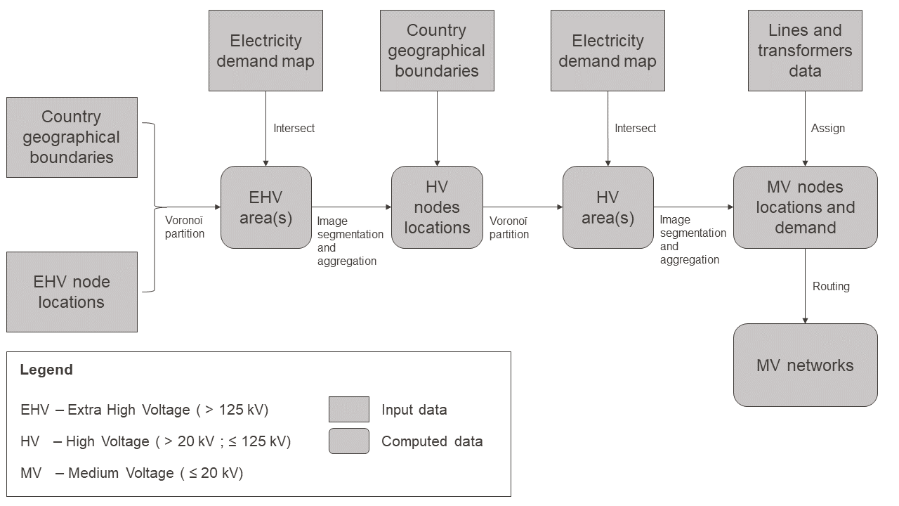
Figure 5.1: Flow chart for the estimation of countrywide models of medium voltage power distribution networks.

Source: (Gupta, Sossan and Paolone, 2020)

5.2 Districts clustering

The districts obtained are examined in turn in the light of a second clustering that looks at the district’s demand and energetic resources. This last step evaluates the similarity of districts concerning their energy flows in and out. Indeed, an energy hub must be characterised by its flow of energy carriers.

The demand is the sum of all the buildings’ demand in the area. It is an output from the QBuildings software. It considers the demand in terms of space heating (SH) (peak power demand [kW] and total annual energy [kWh/y]), domestic hot water (DHW) (peak power demand [kW] and total annual energy [kWh/y]) and electrical demand (total annual energy [kWh/y]). On the other hand, endogenous resources are evaluated. Some of those resources are buildings related and therefore also come from QBuildings output: total annual irradiance [kWh/y] and annual waste in terms of quantity [kg waste/y] and peak power available [kW].
As detailed in Section 4.2, the irradiance considers the available roof area for solar panels and the facade potential with shadowing. In addition to the buildings related resources, the clustering algorithm should also account for the local resources such as the grid infrastructures (gas, power, district heating network) and the geothermal resources. Figure 5.2 wraps up the algorithm’s variables.
The biomass woody and non-woody potential are determined from the Swiss Federal data, openly accessible on geoadmin.ch (SFOE, 2021). The geothermal resources layer is from SIG data, also openly accessible on map.sitg.ch (SITG, 2021).

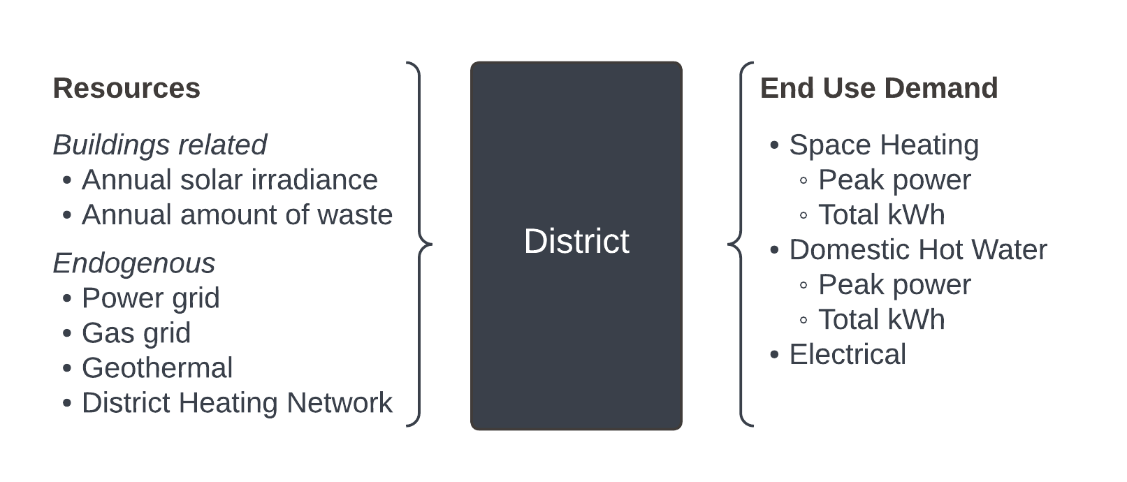
Figure 5.2: Summary of the energy-wise characteristics of a district

The model uses unsupervised clustering algorithms. First, the data goes through a Principal Component Analysis (PCA). The PCA reduces a dataset dimensionality while preserving as much of the variability (i.e. the statistical information) as possible (Jolliffe and Cadima, 2016). It first has been theorised by Pearson (Pearson, 1901) and developed by Hotelling (Hotelling, 1933). The later development in computers opens the possibility to do the computation easily. The goal is to decorrelate the data while maximising the variance. Thus, the old data are expressed as linear functions of the new ones. To do so, the eigenvalues matrix and the eigenvectors are computed. As a result, the new components that reflect the most variance are kept, shrinking the number of dimensions. It also leaves information on the impact of each of the original features on the new ones. It is useful to explain which features have the most significant impact on the clustering decision. The PCA is done in Python using the scikit-learn library (Pedregosa et al., 2011).
The project developed on Python leaves the possibility to use two clustering algorithms, with or without knowing the final number of clusters. A comparison between the two algorithms’ results is further made.

The two methods used are Kmedoids and Gaussian mixture algorithms, described in Section 2.2.

5.2.1 Kmedoids

The cluster number is unknown and so has to be found first.

The algorithm looks for the optimal number of clusters \(K_{opt}\) in between 2 and 30 clusters. The Kmedoids algorithm is performed for each cluster number using the scikit-learn library. The average complexity of the algorithm is \(O(k\cdot n\cdot T)\) with \(k\) the number of clusters, \(n\) the number of samples, and \(T\) the number of iterations. The space complexity is \(O(n^2)\) as pairwise distances are computed and stored in memory (Pedregosa et al., 2011).
The optimal number of clusters is defined according to the scores obtained from the validity indices described in Section 2.2.1. The desired number of iterations \(n_{iter}\) is passed, and the \(K_{opt}\) that comes out on the most occurrences is picked as the final \(K_{opt}\).

def __findkmedoids(self):
    """Gives the ideal number of clusters given a dataset, according to different metrics   (elbow, silhouette, calinski_harabasz) """

    min_c = 2
    max_c = 30

    data = np.array(self.X)
    obj = KMedoids(init='k-medoids++', max_iter=50)
    m1 = vis.KElbowVisualizer(obj, k=(min_c, max_c), metric='distortion')
    m1.fit(data)
    m2 = vis.KElbowVisualizer(obj, k=(min_c, max_c), metric='silhouette')
    m2.fit(data)
    m3 = vis.KElbowVisualizer(obj, k=(min_c, max_c), metric='calinski_harabasz')
    m3.fit(data)
    score_method = [m1, m2, m3]

    return score_method

Once \(K_{opt}\) is known, the clustering can be done. While it was done previously with a faster algorithm to find the optimal \(K_{opt}\) (alternate kmedoids algorithm), the one used here is more demanding (pam kmedoids algorithm).

def __kmedoids(self):
    """Does the KMedoids clustering, returns the clusters, labels and how many data per cluster"""

    samples_per_cluster = []
    data = np.array(self.X)
    obj = KMedoids(n_clusters=self.cnb, init='k-medoids++', method='pam')
    labels = obj.fit_predict(data)
    for j in range(self.cnb):
        samples_per_cluster.append(data[labels == j].shape[0])

    return obj, labels, samples_per_cluster

A stability assessment of the clustering is performed using the Rand index. The labels must first be reordered so that the same clusters are compared every time. The first iteration is taken as a reference, and for every other iteration, the same label is assigned to the cluster with the closest centroid to the first one. The rand index is computed between the first clustering and the others pairwise. The mean index should be higher than the minimum Rand Index defined in Equation (2.2).

def stability_assess(self):
    """Assess to which extent the clustering will give the same results by repeating the experience,
    so to which extent we can trust those clusters """
    # --------------------------------------------------------------------------------------
    # First, we have to relabel the clusters so that cluster 1 always corresponds to 
    # the same one
    # To do so, we measure the distance between centroids, the minimal one is 
    # assigned to the same cluster label
    # This step is actually not essential depending on the metrics we use

    ref_cluster = self.clustering[0].cluster_centers_  
    # 1st as a ref so that everything is renamed after it
    size = ref_cluster.shape[0]
    iter = len(self.clustering)
    labeling = np.zeros((iter - 1, size))
    count_iter = 0
    index: int = 100
    for i in self.clustering[1:]:
        comp_cluster = i.cluster_centers_
        count1 = 0
        for k in ref_cluster:
            min_dist = np.infty
            count2 = 0
            for m in comp_cluster:
                if min_dist > np.linalg.norm(k - m):
                    index = count2
                    min_dist = np.linalg.norm(k - m)
                count2 += 1
            labeling[count_iter][count1] = index
            count1 += 1
        count_iter += 1
    for i in range(1, iter):
        for j in range(self.clustering[i].labels_.shape[0]):
            ini_clust = self.clustering[i].labels_[j]
            sorted_clust = labeling[i - 1][ini_clust]
            self.clustering[i].labels_[j] = sorted_clust

    # -----------------------------------------------------------------------------
    # Now, we can use metrics that compare how do iterations compare to each other
    # Rand index, VI, Jaccard, ...

    ref_labels = self.clustering[0].labels_
    mean_rand = 0
    for i in self.clustering[1:]:
        mean_rand += adjusted_rand_score(ref_labels, i.labels_)
    mean_rand = mean_rand / (iter - 1)

    return mean_rand

5.2.2 Gaussian Mixture

The covariance matrix type and the number of components are the parameters to be determined (see Section 2.2.2).
The GaussianMixture algorithm from the scikit-learn library is used to find the parameters of the GMM model. The different covariance matrices with a number of components \(n\) (that corresponds to the number of clusters \(K\) in the Kmedoids algorithm) varying between 2 and 50 are tested, and the AIC and BIC are used to determine a posteriori which configuration was the best.
The algorithm is implemented with a max number of iterations of 100 before it converges. The function coding the model determination is available below.

    def __findgaussmix(self):
        """Gives the ideal number of clusters given a dataset, according to different
        metrics (AIC, BIC) """

        min_c = 2
        max_c = 20
        bic_score = []
        aic_score = []
        best_bic = np.infty
        best_aic = np.infty
        data = np.array(self.X)
        cv_types = ["spherical", "tied", "diag", "full"]
        for cv_type in cv_types:
            for i in range(min_c, max_c):
                obj = GaussianMixture(n_components=i, covariance_type=cv_type, max_iter=100, reg_covar=1e-5)
                obj.fit(data)
                bic_score.append(obj.bic(data))
                aic_score.append(obj.aic(data))
                if bic_score[-1] < best_bic:
                    best_bic = bic_score[-1]
                    best_gmm_bic = obj
                if aic_score[-1] < best_aic:
                    best_aic = aic_score[-1]
                    best_gmm_aic = obj
        scores = np.array([bic_score, aic_score])
        gmms = np.array([best_gmm_bic, best_gmm_aic])

        return scores, gmms

The data in the input of the algorithm is essential. Indeed, the GaussianMixture model is relatively sensitive to extreme values in the choice of its number of components. If a data item does not fit into the framework of the components, the model will prefer to add one. This property has the advantage of having very stable groups despite outliers once the number of components has been determined, but conversely, this number of components is vulnerable to outliers.  Those considerations lead to a choice of design:

• Either the input to the clustering algorithm remains as it is, with some data further away from the others,
• Or the input data can be processed before the clustering. The extreme values substantially impact the choice of the number of components. It is then possible to process these values by removing them from the data set or by reducing them to a threshold value.
  In the context of the GaussianMixture algorithm, a data from a feature is considered as an outlier if \(|x_{(district,\ feature)}| > 3 \cdot \sigma_{feature} + \mu_{feature}\), i.e. if the value is 3 standard deviation far from the mean of all districts on this feature. Only 0.3% of the values are considered by definition. If the concerned districts are removed, the precision of the clustering to typify districts may increase, but some data are lost. On the other hand, by bringing the outliers to a threshold value (for instance, to 3 standard deviations away from the mean of the gaussian), the reality is torsed, and the algorithms might not give a set of clusters that corresponds to something on the field. It makes it harder to use for further applications, like as an input for the REHO optimiser.
  To help the decision, this work leans on the essay on robust estimation from John Tukey (1960).

“We are likely to think of them as ‘strays’ or ‘wild shots’ […] and to focus our attention on how normally distributed the rest of the distribution appears to be. One who does this commits two oversights, forgetting Winsor’s principle that ‘all distributions are normal in the middle’ and forgetting that the distribution relevant to statistical practice is that of the values actually provided and not of the values which ought to have been provided.”

John Tukey

Especially since the set of districts considered is not that important, the extreme values are valuable as they bring information on cases that may happen only once. For example, one can imagine the airport district in Geneva is very specific. While it would appear as an outlier, it still represents an existing zone type.
As for the modifying of outliers, Tukey reminds it is a draconian measure to take:

“Sets of observations which have been detailed by over-vigorous use of a rule for rejecting outliers are inappropriate since they are not samples.”

John Tukey

In the light of these observations, it is decided to keep the dataset as it is in the method. However, performing a second clustering, having filtered the data beforehand and comparing the two results is interesting.

Once the best model has been determined, the clustering is done with the obtained model parameters. The GaussianMixture algorithm is implemented the same way as previously. The quality of this final clustering is evaluated using the Rand index detailed in (2.1) (code for the index computation is below).

    def stability_assess(self):
        """Assess to which extent the clustering will give the same results 
        by repeating the experience, so to which extent we can trust 
        those clusters """
        # ----------------------------------------------------------------------
        # First, we have to relabel the clusters so that cluster 1 always
        # correspond to the same one
        # To do so, we measure the distance between centroids, the minimal 
        #one is assigned to the same cluster label
        # This step is actually not essential depending on the metrics we use

        ref_cluster = self.clustering[0].means_  
        # 1st as a ref so that everything is renamed after it
        iter = len(self.clustering)
        size = ref_cluster.shape[0]
        labeling = np.zeros((iter - 1, size)) 
        # The idea is to have a table that links the corresponding labels
        count_iter = 0
        index: int = 100
        for i in self.clustering[1:]:
            comp_cluster = i.means_
            count1 = 0
            for k in ref_cluster:
                min_dist = np.infty
                count2 = 0
                for m in comp_cluster:
                    if min_dist > np.linalg.norm(k - m):
                        index = count2
                        min_dist = np.linalg.norm(k - m)
                    count2 += 1
                labeling[count_iter][count1] = index
                count1 += 1
            count_iter += 1
        for i in range(1, iter):
            for j in range(self.labels[i].shape[0]):
                ini_clust = self.labels[i][j]
                sorted_clust = labeling[i - 1][ini_clust]
                self.labels[i][j] = sorted_clust

        # ----------------------------------------------------------------------
        # Now, we can use metrics that compare how do iterations compare
        # to each other
        # Rand index, VI, Jaccard, ...

        ref_labels = self.labels[0]
        mean_rand = 0
        for i in self.labels[1:]:
            mean_rand += adjusted_rand_score(ref_labels, i)
        mean_rand = mean_rand / (iter - 1)

        return mean_rand

The two methods for using the clustering algorithms are implemented through python classes; KmedoidsCluster and GaussianMixtureCluster. Before using the classes, the code normalises the data and runs a PCA. Each class can be called with or without the key clustering parameters (\(K\) the number of clusters for Kmedoids and \(n\) the number of components with the covariance matrix type for GaussianMixture). If called without, classes call the respective method to determine the parameters (findkmedoids or findgaussmix). When the parameters are available, either because they have been passed as an argument or computed, the classes call the clustering algorithm (kmedoids and gaussmix) and assess the stability of the clustering. The method’s code was detailed above in each methodology section.

No objective criteria have been defined for judging the quality of a clustering result. Thus, the clustering validation is done by looking at how good it is working for its initial purpose: the idea was to assimilate a district’s REHO results to all the similar districts. Therefore, the grouping quality is checked by running REHO on districts supposed to be similar and comparing the results.

References

© EPFL-IPESE 2022
Master thesis, Spring 2022
Joseph Loustau