4 QBuildings
As discussed, efficient decision-making tools are needed to enable good energy-wise policies. This challenge is being addressed by optimisation tools development in this project context. Developed in the financial domain, mathematical optimisation has become an important tool in many fields. It helps human decision-making. The user asks for an objective to optimise (e.g. an assets portfolio) under constraints that should model the case (e.g. the maximum budget that can be invested, the interest rate). The complexity of one optimisation can be extremely high, leading to a long computational time or the impossibility of finding an optimal solution. Therefore, the problem has to be stated in a form that is mathematically easier to solve. One of the most popular is the convex optimisation, as the optimum is handy to define. For instance, in Figure 4.1, it is intuitive to find the minimum of the function. Indeed, every local minimum is a global minimum. A problem is said convex if the objective function is convex and the feasible set (defined by the constraints) is convex as well. Its standard form is defined in Equation (4.1).
Figure 4.1: Example of a convex function.
where:
- \(\boldsymbol{x}\) are the decision variables,
- \(f\) is the objective function, convex,
- \(g_i(\boldsymbol{x})\) are the inequality constraints, convex functions,
- \(h_i(\boldsymbol{x})\) are the equality constraints and are affine transformations of form \(h_i(\boldsymbol{x}) = \boldsymbol{a_i} \cdot \boldsymbol{x} - b_i\)
In the context of an energy system optimisation problem, the goal is to minimise an objective function - generally related to overall costs and environmental impact - while satisfying the demand. This project integrates itself into one of those tools, the Renewable Energy Hub Optimiser (REHO). REHO is an ongoing project that embeds different energy conversion and storage technologies and proposes a range of solutions to the problem for each building. It ensures the energy balance of the specified system through the energy demands and physical properties constraints. It can perform multi-objective optimisation (MOO), using Pareto curves, and Key Performance Indicators (KPIs) parametric studies to help decision-making. The optimisation is performed using a Mixed Integer Linear Programming (MILP) model. Linear problems are a subset of convex problems, where the objective function and all the constraints are linear. There are called MP when some variables are constrained to be integers while others are not. To illustrate, when operating an energy conversion unit, it can be either used or not used (0 or 1 value), while how much it is used can vary between its minimum and maximum capacity (0 to 1 value).
REHO enables the optimisation on two scales:
- Building scale, with independent solving of each building,
- District scale, which considers community-wide interactions.
REHO requires as input data on buildings, such as the Energetic Reference Area (ERA), the energy heating, and hot water demand or the building type (see Appendix 12, Table 12.1).
In Switzerland, data sets on buildings are available on a national and regional scale, thanks to works from national administration (e.g. cadaster) or cantonal services. This work uses QBuildings, a software that combines a Geographical Information System (GIS) database with a Python repository, initiated by Luc Girardin in 2012 (Girardin, 2012). The development of such a framework, allowing to aggregate and generate energy-related buildings data, was motivated by several challenges:
- the lack of collaborative platforms where data are grouped with common standards and methods,
- the difficulty in identifying sources of local information and retrieving actual on-site measurements,
- the intensive need for trustful data from the energy transition perspective.
However, the software is not fully operational and cannot integrate information at the local level. Thus, this project recasts QBuildings in version 2.0, where the initial structure is modified to fit the laboratory developments and needs.
The structure of the software can be seen in Figure 4.2. It comprises a database, a python repository, and a file repository for the external data. An SQL database is divided into three schemes (numbers 1, 2, 3). Those schemes are constructed by collecting external data stored on a drive (4). Each database is related to a folder on the drive containing the input layers. Python methods are used to treat each input layer accordingly (5).
Furthermore, outside QBuildings, an interface is provided to visualise the constructed buildings’ GIS data (6).
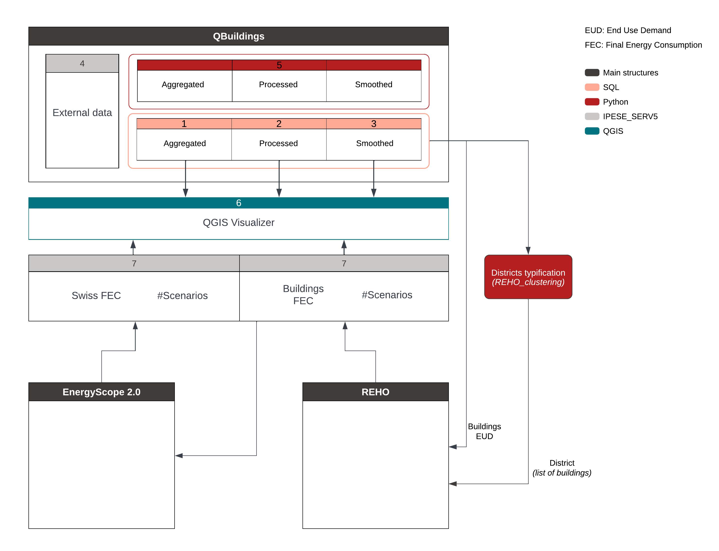
Figure 4.2: Integration of QBuildings with the existing IPESE projects.
4.1 Aggregated
This layer is used to centralise and merge raw data from diffuse information. It starts with data available at the national scale (mandatory) and, if available, uses local data from the area of interest (cities or cantons often have data of their own). Figure 4.3 sums up the minimum set of input layers used to construct a data set. In detail:
- The RegBL is the Swiss federal register of housing and buildings. It catalogues information on buildings, housings and streets. The interest is in the buildings’ information, referenced by street addresses and linked to a Universally Unique Identifier (UUID), named EGID.
- Cadaster refers to swissBuildings3D, a federal data set that describes buildings geometries in three dimensions, with a high degree of detail. It is constructed based on aerial photo-strips (swissBUILDINGS3D 2.0. Federal office of topography swisstopo, no date).
- Sonnendach is a project conducted in Switzerland to build a “solar cadaster”. The data set references every roof and facade in Switzerland and estimates the solar potential and useful surface for each of them (Daniel Klauser, 2016).
- SIA 2024 and SIA 380/1 are standards. SIA 2024 is the standard for Space usage data for energy and building facilities (Brüttisellen-Zurich, 2021), and SIA 380/1 is the standard for Heat requirements for heating (Brüttisellen-Zurich, 2016). These two standards categorise buildings according to their usage: housing (collective or individual), administrative, school, etc., and define typical characteristics for each type of building. A surface normalises the data; the ERA for SIA 380/1 and the net floor area for SIA 2024.
Tables 11.1, from Appendix 11, state all the fields taken from the mandatory layers. Additionally, QBuildings uses meteorological data (external temperatures and solar irradiance) from Meteonorm (J. Remund, 2003).
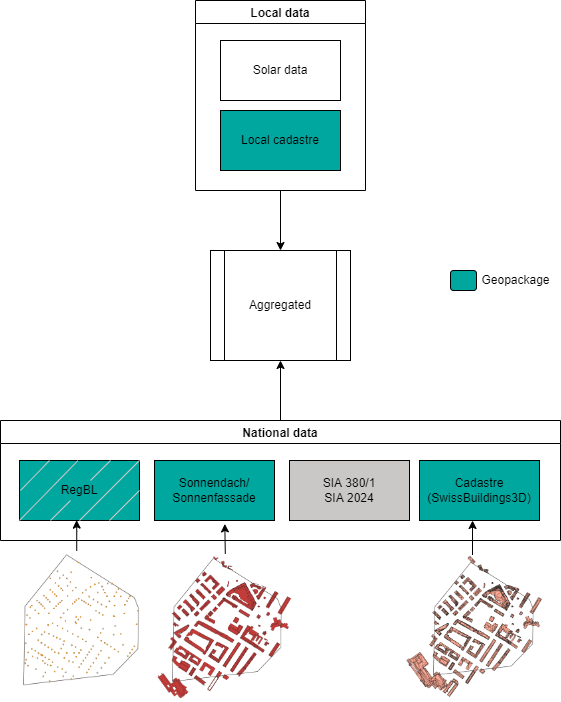
Figure 4.3: Input layers for the aggregated scheme (geographic and others). RegBL is the Swiss national register of housing and buildings. SwissBuildings3D is the national mapping of buildings, in 3 dimensions. Sonnendach is a national database that evaluates the solar potential for roofs and facades.
As Girardin (2012) theorised, “there is a need to combine diverse data sets into an integrated one”. The challenge here is to go from data attached to postal addresses to data referenced by building. Combining the data requires a merge by spatial location, i.e. gathering the GIS geometries that intersect. Figure 4.4 illustrates the different cases and the conflicts that occur between the RegBL that refers to addresses (points, identified by an EGID number) and the cadaster that map the buildings’ geometrical limits (polygons). In the case of multiple EGIDs for one building, the information that refers to EGIDs must then be grouped. An average by area is performed to do so. The area to choose to average the data depends on the data. Indeed, some data sets refer to the Energy Reference Area (ERA) (the area to be heated), others to the net floor area.
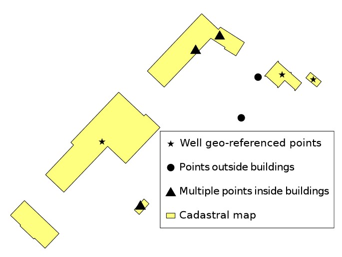
Figure 4.4: GIS View of the badly geo-referenced points to be cleaned and integrated. Source: (Girardin, 2012)
The Aggregated scheme reads all the buildings’ related information. The envelope of buildings is computed thanks to the cadaster. Once the building envelope is available, a spatial join can be done for every data that falls in this envelope. QBuildings Processed layer will need statistical standards related to the category of the building and its year of construction (or renovation, if applicable). Therefore, SIA 380/1 and SIA 2024 are fetched in the Aggregated layer. The data for each type of building are available in Appendix 11, Tables 11.2 and 11.3.
The necessary data for a building are its characteristics, its roofs and facades and the transformer to which it is linked. Each of those pieces of information is stored in a table. At this stage, the data from the RegBL are kept aside. Each table row is identified by a unique primary key. Tables are linked with each other with foreign keys. If other data were to be added, for instance, the geothermal zones to which it belongs, a new table would be created with a primary key linked to another of the existing tables.
The output tables and their fields are explained in Appendix 11, Table 11.4.
4.2 Processed
This layer computes the energy signature of the building, that is, its heating and cooling energy needs and the hot water energy need. The computation is based on a characterisation of the building envelope according to the building class (Residential, Industrial, etc.) and period (<1919, 1919-1930, etc.). This characterisation has been done on a building sample from Geneva in Girardin (2012). The thermal coefficients have been calculated using known heat demands and surfaces and crossed with temperature data. The thermal coefficients are detailed in Figure 4.5.
The data from the buildings tables and the RegBL are grouped, and the corresponding thermal coefficient for each building is identified so that the heating demand can be computed (using hourly temperature data). The SIA data’s ventilation losses, hot water demand, and waste production are also computed with the combined data. Finally, the solar gains are computed using hourly meteorological data over a year.
Figure 4.5: Thermal heating and cooling coefficients for each buildings categories.
Out of the processed schema, the solar potential of the building (irradiance received per year [kWh/y]) is also added. It accounts for the roofs and facades area of the building available for installing PV panels and the annual irradiance each received. The numbers are retrieved from the Sonnendach and Sonnenfassade data (BFE, no date) plus the ones obtained by Walch (2022). A mean is done between the two sources, weighted by the confidence level in the one from Walsh, where the relative error is available.
weight_irr = np.zeros(self.roof.df.index.size)
weight_area = np.zeros(self.roof.df.index.size)
avg_irr = []
avg_area = []
for i, row in self.roof.df.iterrows():
    if not math.isnan(row['egid_walsh']):
        weight_irr[i] = 1-row['mean_annual_irr_kWh_m2_y_std']/row['mean_annual_irr_kWh_m2_y_walsh']
        weight_area[i] = 1-row['area_roof_solar_m2_std']/row['area_roof_solar_m2_walsh']
        avg_irr.append(np.average(row[['mean_annual_irr_kWh_m2_y', 'mean_annual_irr_kWh_m2_y_walsh']],
                       weights=[1-weight_irr[i], weight_irr[i]]))
        avg_area.append(np.average(row[['area_roof_solar_m2', 'area_roof_solar_m2_walsh']],
                        weights=[1 - weight_area[i], weight_area[i]]))
    else:
        avg_irr.append(row['mean_annual_irr_kWh_m2_y'])
        avg_area.append(row['area_roof_solar_m2'])
self.roof.df['mean_annual_irr_kWh_m2_y'] = avg_irr
self.roof.df['area_roof_solar_m2'] = avg_area
It is relevant to highlight that the Sonnendach and Sonnenfassade data have a shadow model (Appendix 11, Figure 11.1). It also estimates the heating and hot water needs by EGID from RegBL data. It is interesting to compare those estimations’ results with those obtained by QBuildings.
The output tables and their fields are described in Appendix 11, Table 11.5.
4.3 Smoothed
The data aggregation from various layers and the computation of new data may have created some extreme values. The data set is smoothed so that the outliers are removed. The energy and hot water signature data, normalised by the energy reference area, are treated. The process used to reduce the effect of the outliers on the data is the Winsorizing (‘Winsorizing’, 2022). It brings back the most extreme values to the quantiles \(\frac{\alpha}{2}\) and \(1 - \frac{\alpha}{2}\) where \(\alpha\) is the tolerance fixed by the user (usually and in this case as well \(\alpha=5\%\)). Therefore, the mean of the data is changed. Figure 4.6 illustrates the data distribution for the energy heating signature within a boxplot. It highlights that the data are widely spread. A much more coherent data set is obtained when winsorising, as seen in Figure 4.7.
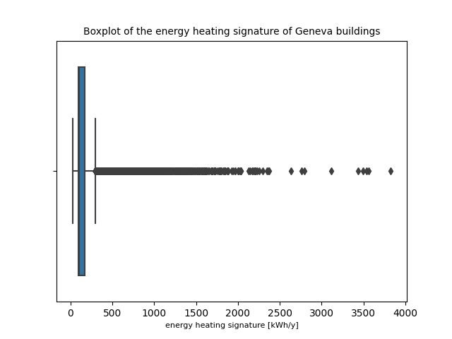
Figure 4.6: Example of a boxplot before the winsorization.
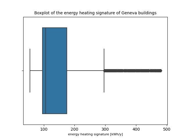
Figure 4.7: Example of boxplot after the winsorization.
QBuildings output tables processed and smoothed have information that can be the input for the districts typification or directly in REHO.
To check the validity if QBuildings results, a case study is done. The chosen area is the Geneva canton. The zone has the significant advantage that the SIG (Services Industriels de Genève) have a lot of data available, making it possible to cross the results from QBuildings. Therefore, a QBuildings database is built on the Canton. The data from the RegBL, swissBuilding3D and Sonnendach are selected for the Geneva Canton. A database QBuildings-Geneva is created - hosted in PostgreSQL and managed with pgAdmin - with the three schemes described. The database is linked to the Python repository thanks to the SQLAlchemy package. The methods are run on Python 3.9, using the geopandas package to produce a dataframe that contains the data set’s geometry component.
References
© EPFL-IPESE 2022
Master thesis, Spring 2022
Joseph Loustau